Rank is a fundamental operation for Succinct Data Structures. It counts the number of set bits up to a given index in a bit array. How can this be done in constant time and sub-linear space?
keywords
data structures succinct2023-06-09
Memory usage is usually an afterthought when it comes to algorithms and data structures. We focus more on speed.
Lately, I’ve been interested in succinct data structures, where size matters just as much as speed.
What does it mean to be succinct? Simply put, it’s the idea that data structures can be squashed down to nearly the smallest possible representation, while still maintaining at least some of their efficient operations.
Usually speed is sacrificed at the expense of space, or vice versa, and so it’s magical that succinct data structures somehow manage to avoid this trade off (I will show that this trade off actually still exists, but it’s impressive how the space complexity can be minimized so much).
However, there’s another dimension: flexibility. It’s fair to say that many succinct data structures sacrifice flexibility. For instance, you may have to be OK with a static, read-only version of your data structure, where mutation is done “offline”. When applied to the right type of problems, this is an acceptable trade off.
Succinct data structures are commonly created using bit arrays, since the usage of typical data types and pointers are too space expensive. There are some fundamental, “building block” operations that are often used. One such operation is called rank.
Given a sequence of bits, B, rank tells you how many set bits there are up to a given position, idx. Since rank is a building block, used to formulate more sophisticated operations, it must be efficient, but not at the expense of much memory. To be classified as succinct, only a sub-linear amount of additional space can be used. The goal is to answer rank queries in constant time, and using no more additional bits than the original bit array (sub-linear space complexity).
idx  0     6     12    18    24
    ┌┴─────┴─────┴─────┴─────┴─────
B   │100110110011011101100111100...
    └┴─────┴─────┴─────┴─────┴─────
┌───┬─────────────┐
│idx│rank₁(B, idx)│
├───┼─────────────┤
│  0│            0│
│  1│            1│
│  6│            3│
│ 12│            7│
│ 18│           11│
│ 24│           15│
└───┴─────────────┘
There are several examples of this for a single machine word on Sean Anderson’s Bit Twiddling Hacks web page, and gcc also has a __builtin_popcount. Computing rank in constant time for an arbitrarily long bit array will require some additional bits to be stored alongside the original array, plus some interesting techniques.
The strategy ends up being clever combination of these three main ideas:
If we were to precompute the answers to rank for each offset in the bit array, then that would be a simple way to have constant time complexity, but it would use an enormous amount of space. It would be far from succinct.
For example, if the precomputed answers are stored using int‘s, that is sizeof(int) * CHAR_BIT bits for each bit in the original bit array – many times more bits than needed.
Assume that all logarithms written as log(n) are base 2: log₂(n). Also note that log²(n) is equivalent to log(n) * log(n).
The first tactic is to encode the precomputed answers using a minimal number of bits. The worst-case scenario is a bit array with all n bits set to 1. It would require only log(n) bits to represent the rank answers for each offset or index in the bit array, rather than sizeof(int) bytes.
    ┌───┬───┬───┬───┬───┬───┬───┐
 B  │   │   │   │   │   │   │   │ n bits
    └───┴───┴───┴───┴───┴───┴───┘
      │   │   │   │   │   │   │
      ▼   ▼   ▼   ▼   ▼   ▼   ▼
    ┌───┬───┬───┬───┬───┬───┬───┐
 R1 │   │   │   │   │   │   │   │ n * log(n) bits
    └───┴───┴───┴───┴───┴───┴───┘
      precomputed rank values
This encoding brings the memory usage to O(n * log(n)) bits for an auxiliary bit array, R1, providing constant-time rank lookups. It’s not succinct though.
The next tactic is to store only a limited number of precomputed answers, rather than storing every single one, in order to save space. Slice up the input data into chunks of size b, and only store answers up to the beginning of each chunk.
The values in R1 are the number of set bits leading up to the corresponding chunk. The values accumulate from chunk to chunk, so we can think of them as cumulative, partial rank query answers.
   ┌────────┬────────┬────────┐
 B │ chunk  : chunk  : chunk  │ n bits
   └────────┴────────┴────────┘
   └──┐   ┌─┘ ┌──────┘
      ▼   ▼   ▼
    ┌───┬───┬───┐
 R1 │   │   │   │ n * log(n) / b bits
    └───┴───┴───┘
     cumulative rank values
This strategy is akin to multiplying two numbers in your head: You may not have 8 * 12 memorized, but you know that 8 * 10 = 80, and that gets you close enough to figure out with your fingers that 8 * 2 = 16, so you reach the final result, 80 + 16 = 96, by doing a quick, memorized lookup, plus a little bit of extra work on your hands.
This obviously reduces the space complexity, but the constant-time lookups are no longer in reach (for now). Two interesting questions to figure out are:
Guy Jacobson, who introduced these concepts in his PhD thesis, “Succinct Static Data Structures”, suggested that the chunks should be b = log²(n) bits.
I’ve been trying to understand why b = log²(n) is the right choice. I think that it boils down to the fact that when you pick b to be a multiple of log(n), then the log(n) term in the numerator vanishes. The result is a sub-linear space complexity:
O(n * log(n) / log²(n)) =

O(n / log(n)) =

ǒ(n)
This is a desired space complexity, but the time complexity is now O(log²(n)), since we need to scan up to an entire chunk to find the answer. There are more tricks to employ before we can get back to constant query time.
Jacobson also suggested that a two-level auxiliary bit array scheme could improve the query time, while still maintaining sub-linear space complexity. At the top level, we have R1, which stores precomputed answers up to each chunk of size, b, just as explained so far. Another auxiliary bit array, R2, can be used in a similar fashion as R1. Values in R2 are also partial answers, but relative to each chunk.
Values in R1 correspond to chunks of size log²(n) from B. Values from R2 correspond to sub-chunks from B of size 1/2 * log(n).
Since values in R1 can approach n, the total number of bits, they are encoded using log(n) bits. However, for R2, the values approach b, the size of a chunk, so each value can be encoded using even fewer bits: log(b).
     [more rank values, relative to a chunk]
    ┌───┬───┬───┬───┬────
 R2 │   │   │   │   │ ... n * log(b) / 2 * log(n) bits
    └───┴───┴───┴───┴────
      ▲   ▲   ▲   ▲   ▲
   ┌──┘   │   │   │   │
   │  ┌───┘   │   │   │ ...
   │  │  ┌────┘   │   │
   │  │  │  ┌─────┘   │
   │  │  │  │  ┌──────┘
   ┌──┬──┬──┬──┬──┬──┬──┬──┬──┐
 B │ chunk  : chunk  : chunk  │ n bits
   └──┴──┴──┴──┴──┴──┴──┴──┴──┘
   └──┐   ┌─┘ ┌──────┘
      ▼   ▼   ▼
    ┌───┬───┬───┐
 R1 │   │   │   │ n * log(n) / b bits
    └───┴───┴───┘
     [cumulative rank values]
Armed with the second auxiliary bit array, the time complexity has improved to be O(log(n)). That’s because we can now perform two constant-time table lookups into R1 and R2, and then do a linear scan of the remaining bits in B, which will never be more than the size of a sub-chunk. The space required for R2 is also sub-linear.
O(n * log(b) / 2 * log(n)) =

O(n * log(b) / log(n)) =

O(n * log(log²(n)) / log(n)) =

O(n * log(2 * log(n)) / log(n)) =

O(n * log(log(n)) / log(n)) =

ǒ(n)
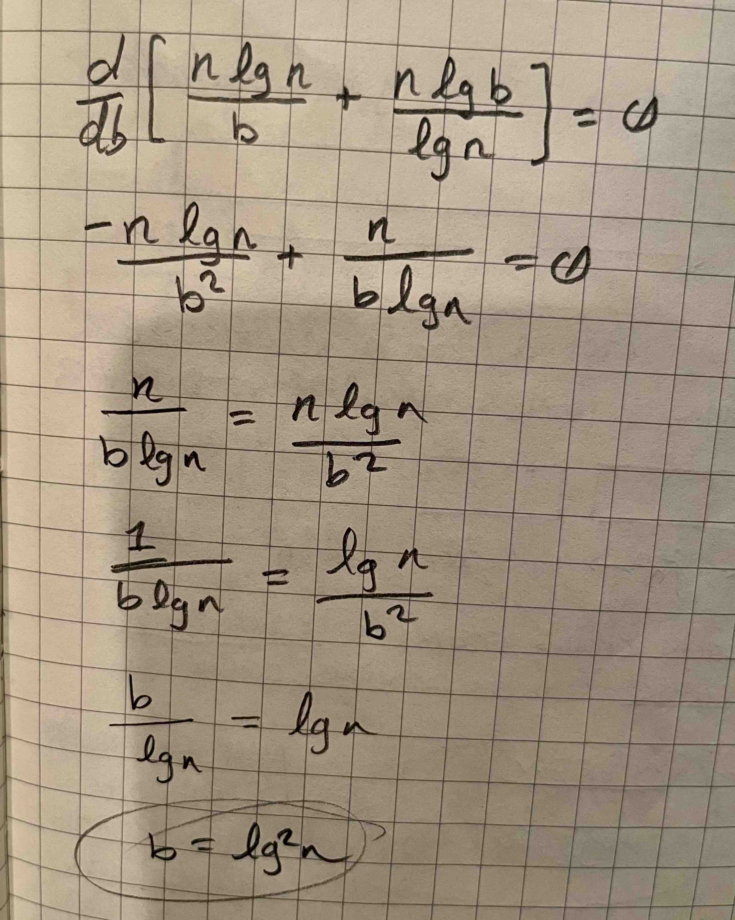
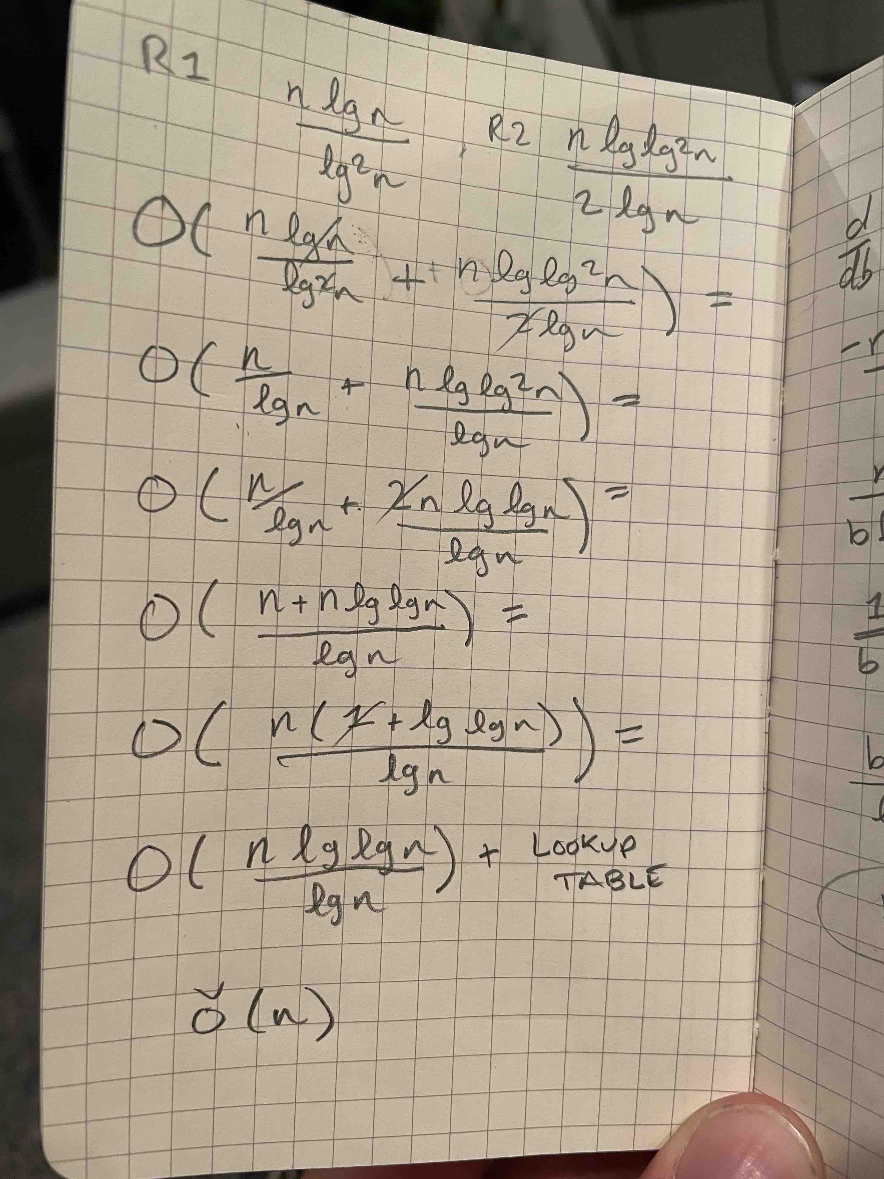
There’s an interesting relationship between R1 and R2, with respect to b. As the chunk size increases, there are fewer chunks overall, meaning less data stored in R1. However, that also means that more values are stored in R2. In other words, if the n log n / b term shrinks, then the n log b / log n grows larger. We can show that the optimal choice for b is in fact log²(n) using some calculus (Big thanks to Keith Schwarz for showing me how to do this.)
As for getting down to constant query time, the final trick is to consider how few bits there are within each sub-chunk.
Just to put things into perspective, assume that the bit array is under n = 2^128 bits long (a really big number), and that the processor’s word length is 64 bits. In this case, a single call to __builtin_popcountll should suffice, and we can consider this constant time. If n were to be greater than roughly 2^128, then a sub-chunk of 1/2 * log(n) would have more bits than a machine word, and a lookup table containing all possible values can be used instead.
Since the values in the lookup table are relatively small, and highly redundant, a lot of space can be saved. For example, assume that the x = 1/2 * log(n) = 4 sized sub-chunks comes out to 4 bits each (for demo purposes). That would mean that there are 2ˣ = 2⁴ possible sequences of bits that a sub-chunk could be:
0000 0001 0010 0011
0100 0101 0110 0111
1000 1001 1010 1011
1100 1101 1110 1111
The target index to rank₁(B, idx) probably won’t line up directly with a sub-chunk, so we need to store answers for each offset into each of these 2⁴ bit sequences. The answers are represented using log(x) bits. The math works out to be a sub-linear amount of space as well, due to the size of the sub-chunk, x.
- 2ˣ possible bit sequences
- x number of offsets
- log(x) bits to encode an answer

O(2ˣ * x * log(x)) =

O(2^(1/2 * log(n)) * 1/2 * log(n) * log(1/2 * log(n))) =

O(√n * log(n) * log(log(n))) =

ǒ(n)
Now it’s finally possible to find rank in constant time and using fewer bits than the original bit array. The final space complexity comes out to be O(n * log log n / log n), which is sub-linear. The process to find rank₁(B, idx) is as follows:
index / log²(n). Use the chunk index to lookup the partial, cumulative rank value in R1. index / ((1/2) * log(n)). Use the sub-chunk index to lookup the partial, relative rank value in R2. This sounds good in theory, but how does it hold up in practice? I don’t have a good answer to that today. I know that it is super tedious to code this up, though, because of all the bitwise operations, and because of how values are encoded (incomplete demo code here - beware I’m no C programmer).
Rank may not seem too useful on its own, but it’s a key part of more sophisticated operations on succinct data structures. In Jacobson’s thesis, he showed how it can be used to navigate trees and graphs. It’s also a key part of Wavelet Trees, a data structure used to work with compressed text.
Succinct data structures have their place wherever there’s a need to interact with large data sets. Gonzalo Navarro gives one example [¹]:
[…] the DNA of a human genome […] requires slightly less than 800 megabytes if we use only 2 bits per base (A, C, G, T), which fits in the main memory of any desktop PC. However, the suffix tree, a powerful data structure used to efficiently perform sequence analysis on the genome, requires at least 10 bytes per base, that is, more than 30 gigabytes.
So, succinct data structures offer a way to overcome this sort of problem.
Finally, here are some useful links and references to check out if this sort of thing is also interesting to you:
Special thanks to Keith Schwarz, who went out of his way to help me understand how to mathematically show that b = log²(n) is the optimal choice of b.